SVM

Support Vector Machines (SVM) is a supervised learning algorithm used for classification, regression, and outlier detection. Support vector machines focus only on the points that are the most difficult to tell apart, whereas other classifiers pay attention to all of the points.

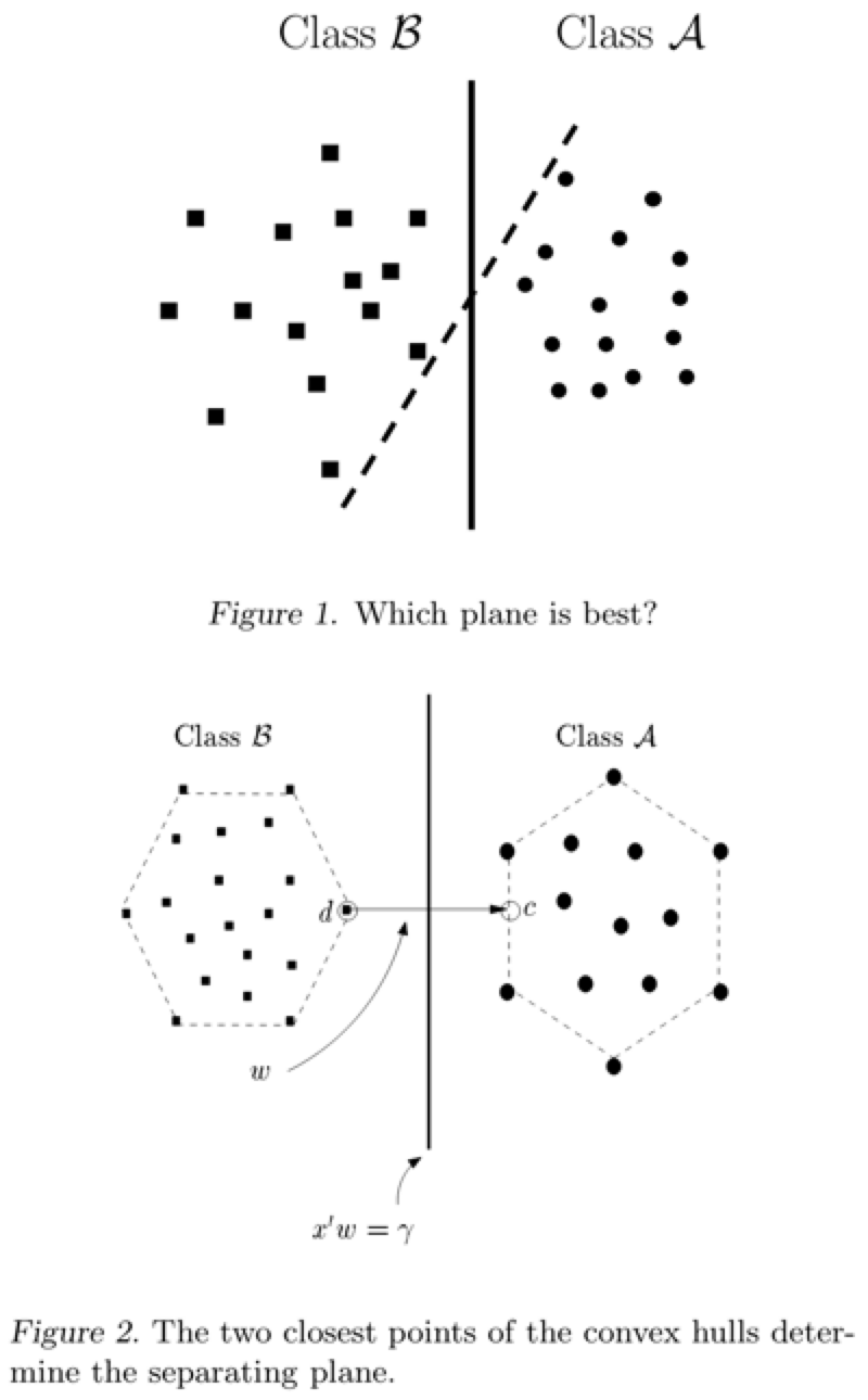
The intuition is that if a classifier is good at separating the most challenging points (that are close to each other), then it will be even better at separating other points. SVM searches for the closest points, so-called “support vectors” (the points are like vectors and the best line “depends on” or is “supported by” them).
Then SVM draws a line connecting these points. The best separating line is perpendicular to it.

Mathematical Formulation

For a binary classification problem:

1. Linear SVM: Minimize: $\frac{1}{2}||w|{|}^2$ Subject to: $y_i(w\cdot x_i+b)\ge 1$ for all $i$
2. Soft Margin SVM (allowing some misclassifications): Minimize: $\frac{1}{2}||w|{|}^2+C{\sum }_{i=1}^n{\xi }_i$ Subject to: $y_i(w\cdot x_i+b)\ge 1-{\xi }_i$ and ${\xi }_i\ge 0$ for all $i$.
   SVM optimization problem can be rewritten as $\frac{1}{2}||w|{|}^2+C\ast \Sigma max(0,1-y_i(w\cdot x_i+b))$ - the sum of hinge losses for all training examples.

Where:

• $w$ is the normal vector to the hyperplane
• $b$ is the bias
• $C$ is the regularization parameter
• ${\xi }_i$ are slack variables

Kernel Trick

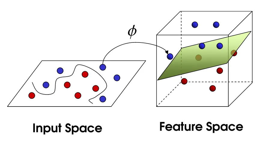
The idea is that the data, that isn’t linearly separable in the given $n$ dimensional space may be linearly separable in a higher dimensional space.

The kernel trick provides a solution. The “trick” is that kernel methods represent the data only through a set of pairwise similarity comparisons between the original data observations $x$ (with the original coordinates in the lower dimensional space), instead of explicitly applying the transformations $\varphi (x)$ and representing the data by these transformed coordinates in the higher dimensional feature space.

In kernel methods, the data set $X$ is represented by an $n\cdot n$ kernel matrix of pairwise similarity comparisons where the entries $(i,j)$ are defined by the kernel function: $k(xi,xj)$. This kernel function has a special mathematical property. The kernel function acts as a modified dot product.

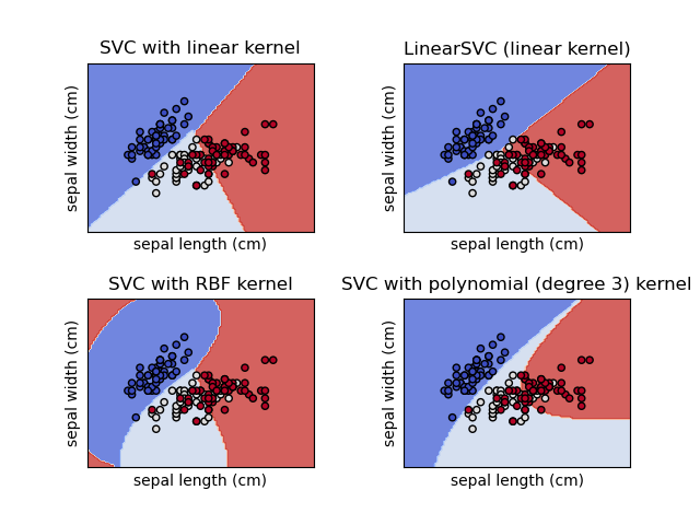
1. Linear: $K(x_i,x_j)=x_i\cdot x_j$
2. Polynomial: $K(x_i,x_j)=(\gamma x_i\cdot x_j+r{)}^d$
3. RBF (Gaussian): $K(x_i,x_j)=exp(-\gamma ||x_i-x_j|{|}^2)$
4. Sigmoid: $K(x_i,x_j)=tanh(\gamma x_i\cdot x_j+r)$
   

Advantages

• Effective in high-dimensional spaces
• Memory efficient as it uses only support vectors
• Versatile through different kernel functions
• Robust against overfitting

Disadvantages

• Sensitive to the choice of kernel and regularization parameter
• Does not directly provide probability estimates (requires additional methods like Platt Scaling, significantly increases computation cost)
• Can be computationally intensive for large datasets

Code example

import numpy as np
 
class SVM:
    def __init__(self, learning_rate=0.001, lambda_param=0.01, n_iters=1000):
        self.lr = learning_rate
        self.lambda_param = lambda_param
        self.n_iters = n_iters
        self.w = None
        self.b = None
 
    def fit(self, X, y):
        n_samples, n_features = X.shape
        y_ = np.where(y <= 0, -1, 1)
 
        self.w = np.zeros(n_features)
        self.b = 0
 
        for _ in range(self.n_iters):
            for idx, x_i in enumerate(X):
                condition = y_[idx] * (np.dot(x_i, self.w) - self.b) >= 1
                if condition:
                    self.w -= self.lr * (2 * self.lambda_param * self.w)
                else:
                    self.w -= self.lr * (2 * self.lambda_param * self.w - np.dot(x_i, y_[idx]))
                    self.b -= self.lr * y_[idx]
 
    def predict(self, X):
        linear_output = np.dot(X, self.w) - self.b
        return np.sign(linear_output)

Links:

• A great visualization
• Sklearn documentation
• Duality and Geometry in SVM Classifiers
• The explanation of the kernel trick